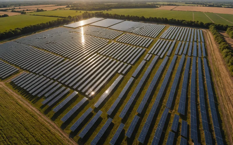
A plant's expected production curve shows what it could generate when panels operate at nameplate efficiency under the period's irradiance and temperature. Its actual curve shows what it produced. The difference is not random noise. It combines the loss mechanisms affecting the asset now. Properly separating those losses helps an O&M program target issues that matter instead of spending inspection time and money where they will have little effect.
Generation gap analysis isolates underperformance by place and time. A useful result says more than a plant is 4 percent below expected. It can show that 1.5 percent comes from soiling on the eastern sub-array, 0.8 percent from clipping on three inverters with high DC/AC ratios, and 1.7 percent from partial shading by perimeter vegetation that grew after commissioning. Each cause carries its own remediation cost and O&M owner.
Expected Energy and Actual Energy: The Building Blocks
A defensible expected energy estimate comes before any gap measurement. Many monitoring systems introduce their first major error here. PR calculations based on nameplate module power, a fixed irradiance reference, and data sheet temperature coefficients offer a reasonable baseline, but systematic errors can enter at every level.
Module output declines with age. By its fifth year, a plant using typical mono-PERC or TOPCon panels has probably lost 1.5 to 2.5 percent from nameplate, with the loss spread unevenly through the array. If the model still uses nameplate values, comparisons carry that accumulated bias. Expected output is overstated, so the measured gap appears larger than it really is.
Irradiance measurement creates another error source. A pyranometer or reference cell that has drifted, accumulated soiling, or shifted by even a few degrees in tilt may no longer represent the light reaching the panels. In plants that have gone several years without recalibrating the irradiance reference, this is one of the most frequent causes of false gaps.
Temperature adjustment is often underweighted in monitoring systems. Silicon panels lose about 0.3 to 0.45 percent of output for each degree Celsius above STC. On a summer day in northeastern Brazil, module temperatures may reach 65 to 70 degrees Celsius. A measured PR of 78 percent with a 68-degree-module is normal; the same 78 percent PR with a 30-degree-module indicates underperformance of 5 to 8 percent against a realistic expectation.
Breaking Down the Gap: Plant to String
A fleet-level underperformance figure helps with benchmarking and contract compliance, but it cannot tell you where to send a technician. Effective gap analysis requires progressively finer decomposition.
Begin at plant level with a weather-corrected energy index: actual energy divided by expected energy for the measured irradiance and temperature during the period. This removes variables outside your control. An index of 0.94 means the plant is producing 94 percent of what physics predicts. The next task is explaining the 6 percent.
Then compare the weather-corrected energy index between inverters. If one or two consistently lag the rest of the fleet, that pattern merits isolation. Possible causes include inverter clipping, discussed below, systematically heavier soiling in one zone, or a degraded MPPT channel.
At string level, compare current and power within each inverter after normalizing for temperature and irradiance. This can reveal strings lowering inverter output. Check whether the loss is concentrated in one geographic zone, which suggests soiling or shading; spread evenly across the array, which suggests an issue such as an incorrect irradiance reference or module degradation; or limited to isolated strings scattered across the plant, which suggests individual faults.
Each pattern calls for a different investigation. A concentrated zone may require a cleaning route or shade survey. Uniform loss across strings points toward calibration or genuine PR drift. Isolated string anomalies call for fault detection.
Time-of-Day and Seasonal Breakdown
Timing can be as informative as location. A gap limited to early morning and late afternoon, when sun angles are low, fits a soiling or incidence-angle modifier pattern. A gap limited to peak irradiance, roughly 10 AM to 2 PM, points to clipping: the inverter rejects DC power once it exceeds rated capacity at high irradiance.
Gap patterns also shift with the sun's seasonal path. Shading that is minor in summer, when the sun is high, can become significant in winter as lower sun angles create longer shadows. An O&M program that treats all seasons alike can miss this loss entirely.
Consider a 20 MW ground-mount plant in Minas Gerais with a perimeter row of eucalyptus trees that grew 3 meters after installation. In December, winter shading on the eastern rows between 7 and 9 AM might represent 0.4 percent of annual generation. On a plant producing 30,000 MWh per year, that is roughly 120 MWh, enough to compare with the cost of vegetation management.
Performance Ratio as a Diagnostic Tool, Not a Report Metric
PR is often reported as one monthly or annual figure, which works for contract compliance and benchmarking. As a diagnostic measure, however, aggregated PR offers little guidance. A single plant-level value shows underperformance but not its cause, location, or timing.
Diagnostic PR analysis separates the metric into components. Compare PR at string and inverter levels. Review its hour-by-hour movement. Check how the trend changed over the last six months and whether it is accelerating or stable. Also ask whether some plant sections have declined more than others.
When Solarvyew onboards a plant, we first produce a time-resolved PR surface in many cases: PR for each time-of-day and date combination over the trailing 12 months. Its patterns can be visible immediately and may identify the issue by themselves. A dip every 30 to 45 days that clears within a few days points strongly to irregular cleaning cycles. A progressive year-on-year drift during the dry season fits soiling accumulation.
Connecting the Gap to Revenue
Revenue impact ultimately guides remediation. A 2 percent gap at a plant selling power for BRL 280 per MWh and generating 50,000 MWh each year equals roughly BRL 280,000 in forgone annual revenue. That context helps determine whether a soiling campaign or vegetation management program justifies its cost.
This analysis is illustrative, not a guaranteed projection. Gaps usually have several causes, and some cannot be recovered economically. Panel aging creates inherent degradation that hardware replacement may be needed to reverse. Permanent-structure shading cannot be corrected through O&M alone. Recoverable losses are always less than the total gap, so rigorous analysis separates actionable losses from structural ones.
For recoverable losses, gap analysis becomes a prioritized set of O&M work orders: which sub-arrays to clean first, which strings to inspect physically, and which inverter zones to review for clipping. This link between analytics and field work is where the analysis earns its value. Without it, the figures remain a report metric instead of an operational tool. For a closer look at how soiling appears in gap analysis, read the article on soiling loss at remote sites for a deeper treatment.